Beyond the Formula, A Framework for Value
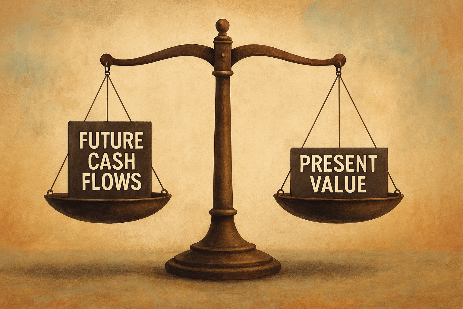
In the world of finance, where market sentiment can be fleeting and prices can swing wildly, a disciplined valuation approach is the most reliable anchor. The Discounted Cash Flow (DCF) model is not just a calculation; it is a powerful framework that cuts through the noise to estimate an asset’s true, or “intrinsic,” value. It operates on a simple yet profound principle: a business’s value is the present value of all its future cash flows. A rock-solid DCF model, however, is not built by chance; it is a product of meticulous execution and a deep understanding of its core components and their interplay.
This report will explore nine proven strategies that move beyond the basics, empowering any analyst to build a DCF model that is not only mathematically correct but also robust, defensible, and truly insightful.
- Start with the Blueprint: The Unlevered Free Cash Flow (FCF) Foundation.
- Define Your Time Horizon: The Explicit Forecast Period.
- Harness the Power of the Discount Rate: Mastering WACC.
- Conquer the Terminal Value: The Two-Method Approach.
- Ground Your Assumptions in Reality: Avoiding the “Garbage In, Garbage Out” Trap.
- Perform Rigorous Stress Testing: The Power of Sensitivity Analysis.
- Uncover the True Value: Bridging Enterprise and Equity Value.
- Avoid Common Pitfalls: A Checklist for Flawless Modeling.
- Conduct Sanity Checks: Validating Your Results Against Reality.
The Strategies
Strategy 1: Start with the Blueprint: The Unlevered Free Cash Flow (FCF) Foundation
Free cash flow, or FCF, is a crucial indicator of a business’s financial health, representing the money left over after a business pays its operating expenses and capital expenditures. For a DCF valuation, the most common and theoretically sound approach is to use unlevered free cash flow, also known as Free Cash Flow to the Firm (FCFF). This metric represents the cash available to all of a company’s capital providers—both debt and equity holders—before any interest payments are made. This is distinct from levered free cash flow, which accounts for cash flow only to equity holders after debt obligations have been met.
To build this foundational cash flow stream, an analyst must begin with a company’s historical financial statements and project its future performance based on a clear understanding of its business model. The formula for unlevered FCF is the core of this process:
FCF=EBIT×(1−tax rate)+D&A−Capital Expenditures−Changes in Net Working Capital
Each component serves a specific purpose in translating a company’s accounting profits into a true measure of its cash generation. EBIT (Earnings Before Interest and Taxes) provides a clean view of the company’s operating profitability. Depreciation and Amortization (D&A) are then added back because they are non-cash expenses that reduce reported earnings but do not involve an actual outflow of cash. Capital Expenditures (CapEx) for long-term investments and changes in Net Working Capital (∆NWC), which reflects cash tied up in day-to-day operations, are subtracted as they represent real cash outflows.
The choice to use unlevered FCF is not arbitrary; it is a critical decision that must be consistent with the discount rate chosen for the valuation. Unlevered FCF measures the cash flow before debt payments, which is a return to both debt and equity providers. Therefore, this cash flow stream must be discounted by the Weighted Average Cost of Capital (WACC), which is a blended rate that accounts for the cost of both debt and equity. A fundamental error in DCF modeling is a mismatch between the type of cash flow being discounted and the discount rate used. By beginning the model with unlevered FCF and committing to the WACC as the discount rate, an analyst establishes a theoretically sound and defensible foundation.
|
Key Components of Unlevered Free Cash Flow (FCFF) |
|
|---|---|
|
Component |
Description and Rationale |
|
EBIT (Earnings Before Interest and Taxes) |
Measures operating profit from core business activities, excluding financing costs and taxes. It is the starting point for understanding a company’s earnings from operations. |
|
Tax Rate |
The tax rate the company is expected to face on its earnings. EBIT is multiplied by (1 – tax rate) to arrive at Net Operating Profit After Taxes (NOPAT). |
|
Depreciation & Amortization (D&A) |
Non-cash expenses that are added back to NOPAT. While they reduce a company’s taxable income, they do not represent an actual outflow of cash. |
|
Capital Expenditures (CapEx) |
Cash outflows for long-term investments in physical assets like property, plant, and equipment. These are real costs necessary to maintain and grow the business and are therefore subtracted. |
|
Changes in Net Working Capital (∆NWC) |
The change in a company’s current assets and liabilities from one period to the next. This accounts for cash tied up in or released from operations (e.g., inventory, accounts receivable) and is subtracted if it’s an increase in assets. |
Strategy 2: Define Your Time Horizon: The Explicit Forecast Period
A DCF model is typically built in two stages: an explicit forecast period (Stage 1) followed by a terminal value (Stage 2). The explicit forecast period is a crucial component where an analyst projects a company’s financial statements in detail, including cash flows, for a defined number of years. For a mature company, this period is often set at five years, but for companies with more unpredictable cash flows or those in high-growth phases, a 10-year or even longer forecast may be necessary to capture their growth trajectory.
One of the most common errors in DCF modeling is choosing a forecast horizon that is too short, a decision that can lead to a severely misleading valuation. The underlying problem is that the DCF model’s terminal value, which represents all future cash flows beyond the explicit forecast, can account for a massive portion of the total valuation—often 50% to 75%. If a company is still in a high-growth phase at the end of a short forecast period, a premature shift to the terminal value will misrepresent its long-term potential. This forces the analyst to either use an unrealistically high terminal growth rate or to severely undervalue the business.
The length of the explicit forecast is therefore not a fixed rule but a strategic decision that must be tailored to the company’s business lifecycle. A technology startup with a rapid growth curve and significant future reinvestment needs will require a much longer and more detailed forecast than a stable, mature utility company. By extending the explicit period to capture the full arc of a company’s high growth and subsequent normalization, an analyst can build a more accurate and robust model.
Strategy 3: Harness the Power of the Discount Rate: Mastering WACC
The discount rate is a fundamental concept in DCF analysis, serving as the rate at which future cash flows are reduced to their present value. It is designed to account for two critical factors: the time value of money (the principle that a dollar today is worth more than a dollar in the future) and the inherent riskiness of the investment. When performing an unlevered DCF, the appropriate discount rate to use is the Weighted Average Cost of Capital, or WACC.
WACC represents the average return required by all of a company’s capital providers—both debt holders and equity holders—weighted by their proportion in the company’s capital structure. The full formula for WACC is:
WACC=(Debt+EquityDebt)×rdebt×(1−tax rate)+(Debt+EquityEquity)×requity
In this formula, r_equity is the cost of equity, which is the return shareholders require to invest in the company’s stock, and is often determined using the Capital Asset Pricing Model (CAPM).
r_debt is the cost of debt, which represents the interest rate a company pays on its debt. The (1 – tax rate) component reflects the tax shield on interest payments, which makes debt a less expensive source of financing for the firm.
The discount rate is arguably the single most influential variable in a DCF model, and even small changes can lead to massive swings in the final valuation. This is because the DCF formula compounds the discount rate over a multi-year period, and the overwhelmingly large terminal value is also heavily dependent on this rate. As the discount rate is in the denominator of the present value calculation, a small increase will cause a disproportionately large decrease in the final valuation. This “sensitivity” is not a flaw of the DCF model but rather a feature that underscores the importance of a meticulously calculated WACC and the need for sensitivity analysis around it. It forces the analyst to confront the high-stakes nature of this single number.
|
Components of a WACC Calculation |
|
|---|---|
|
Component |
Derivation |
|
Cost of Equity ($r_{equity}$) |
The return required by equity shareholders. Typically derived using the Capital Asset Pricing Model (CAPM) or another risk and return model. |
|
Cost of Debt ($r_{debt}$) |
The interest rate a company pays on its debt. Can be derived from the company’s credit rating or the yield on its outstanding bonds. |
|
Tax Rate |
The effective tax rate applied to the company’s earnings. It is used to calculate the tax shield benefit of debt financing. |
|
Capital Structure Weights ($frac{Debt}{Debt + Equity}, frac{Equity}{Debt + Equity}$) |
The proportion of debt and equity in the company’s financing mix. This should reflect the market value of each component. |
Strategy 4: Conquer the Terminal Value: The Two-Method Approach
Since projecting cash flows indefinitely is impractical, analysts must calculate a lump-sum “terminal value” that represents the worth of all future cash flows beyond the explicit forecast period. This terminal value is immensely significant, often accounting for 50% to 75% of the total DCF valuation , which makes its calculation a key determinant of the final result.
There are two widely accepted methods for calculating terminal value: the Perpetuity Growth Method and the Exit Multiple Method.
- Perpetuity Growth Method: This approach assumes the company will continue to generate cash flows indefinitely at a stable, perpetual growth rate (g). The formula is: TV=WACC−gFCFn×(1+g) where FCFn is the free cash flow for the last year of the explicit forecast period. The growth rate g should be conservative and generally align with or be slightly below the long-term, inflation-adjusted growth rate of the economy, typically in the range of 2-3%. An assumption of growth exceeding 5% in perpetuity is considered highly unrealistic.
- Exit Multiple Method: This method assumes the business will be sold at the end of the forecast period for a market-based multiple of a financial metric, such as Enterprise Value to EBIT (EV/EBIT) or Enterprise Value to EBITDA (EV/EBITDA). The formula is: TV=Terminal Multiple×Statistic from Last Forecast Year The multiple is typically based on the trading multiples of comparable public companies or recent transaction multiples.
A crucial best practice is to always cross-check the results of both terminal value methods. The two approaches, while seemingly different, are two sides of the same coin. A specific market-based exit multiple inherently implies a certain perpetual growth rate. If an analyst calculates the terminal value using an exit multiple, they should then back-calculate the “implied g” that would be required to achieve that value with the perpetuity method. If the implied growth rate is unrealistically high (e.g., above 5%), it indicates that the chosen exit multiple is overly optimistic and not aligned with the fundamental perpetual growth assumption. This dual validation ensures that the market-based assumptions are consistent with the fundamental-based assumptions, leading to a more accurate and defensible valuation.
|
Comparing Terminal Value Calculation Methods |
||
|---|---|---|
|
Feature |
Perpetuity Growth Method |
Exit Multiple Method |
|
Underlying Assumption |
The company will continue to grow at a stable rate indefinitely. |
The company will be valued by the market at a certain multiple at the end of the forecast. |
|
Formula |
TV=WACC−gFCFn×(1+g) |
TV=Multiple×Last Year’s Metric |
|
Key Input |
The stable, perpetual growth rate (g). |
The exit multiple (e.g., EV/EBITDA, EV/EBIT). |
|
Best Use Case |
Best suited for stable, mature companies in non-cyclical industries. |
Best suited for valuing a company in an M&A context where a clear exit is contemplated. |
|
Pros/Cons |
Pros: Based on fundamentals, less susceptible to short-term market fluctuations. Cons: Highly sensitive to the growth rate assumption and requires a subjective guess for g. |
Pros: Reflects current market sentiment and peer valuations. Cons: Susceptible to market volatility and may not reflect intrinsic value. |
Strategy 5: Ground Your Assumptions in Reality: Avoiding the “Garbage In, Garbage Out” Trap
A DCF model’s greatest strength—its reliance on fundamental business drivers—is also its primary weakness. The valuation is highly sensitive to the discretionary assumptions an analyst makes about a company’s future performance, which can be subjective and prone to bias. This phenomenon is often summarized by the maxim “garbage in, garbage out,” where unrealistic inputs lead to an equally flawed output.
To avoid this trap, key assumptions must be grounded in reality and supported by a thorough analysis of a company’s historical performance, industry trends, and management plans. This includes all major operating assumptions, such as revenue growth, profit margins, and cost structures, which should be projected with a nuanced understanding of the business and its competitive environment.
Reinvestment assumptions, particularly Capital Expenditures (CapEx) and changes in Net Working Capital (∆NWC), are also critical to get right. A common mistake is to assume high revenue growth without linking it to the necessary capital investments and changes in working capital needed to support that growth. This error can create “value for free” and severely overstate the company’s cash-generating ability. The discount rate and its components also require careful selection, based on the company’s specific risk profile and its capital structure.
The “garbage in, garbage out” problem is magnified by the compounding nature of small, early-stage errors in the forecast. The uncertainty in cash flow projections naturally increases with each passing year, and projections for outer years are often based on the assumptions of preceding years. This means that a small, erroneous assumption in the first year—such as an optimistic revenue growth rate—can amplify variances in later years and lead to a wildly different terminal value. Therefore, the most critical work in building a reliable DCF model is not the final calculation but the painstaking process of creating detailed, defensible projections for the explicit forecast period.
Strategy 6: Perform Rigorous Stress Testing: The Power of Sensitivity Analysis
A DCF valuation should never be viewed as a precise, final number; it is an estimate. Presenting a single-point valuation can create a false sense of accuracy and lead to overconfidence in an investment decision. A more robust approach involves stress-testing the model through sensitivity analysis to provide a defensible valuation range.
Sensitivity analysis involves systematically changing key assumptions to see how the final valuation is affected. The most influential variables to sensitize are the Weighted Average Cost of Capital (WACC), the terminal growth rate, and the revenue growth rate, as minor adjustments to these inputs can have a material impact on the result. This process can be performed manually or by using Excel’s data table functionality, which allows for a dynamic analysis of multiple assumptions at once.
Beyond simply providing a range, the act of performing a sensitivity analysis is a critical diagnostic tool that reveals which inputs are the primary drivers of the valuation and highlights the riskiest assumptions. For example, by creating a sensitivity table that plots a range of WACC values against a range of terminal growth rates, an analyst can visually see the full spectrum of possible outcomes. If a small change in a single variable causes a disproportionately large swing in the valuation, it signals that the investment is highly sensitive to that specific risk. This provides a clear, quantitative basis for discussing risk and can help guide an investment decision. It forces the analyst to be proactive and transparent rather than reactive to unexpected market movements.
|
DCF Valuation Sensitivity Analysis (in $M) |
|||||
|---|---|---|---|---|---|
|
WACC |
Terminal Growth Rate |
||||
|
2.0% |
2.5% |
3.0% |
3.5% |
4.0% |
|
|
8.0% |
$1,250 |
$1,375 |
$1,520 |
$1,695 |
$1,900 |
|
8.5% |
$1,150 |
$1,260 |
$1,385 |
$1,525 |
$1,680 |
|
9.0% |
$1,060 |
$1,160 |
$1,265 |
$1,380 |
$1,510 |
|
9.5% |
$980 |
$1,070 |
$1,165 |
$1,260 |
$1,370 |
|
10.0% |
$910 |
$995 |
$1,080 |
$1,165 |
$1,265 |
Strategy 7: Uncover the True Value: Bridging Enterprise and Equity Value
The unlevered DCF approach calculates a company’s Enterprise Value (EV), which represents the total value of the business, encompassing both debt and equity. However, for most investors, the ultimate goal is to determine the Equity Value—the portion of the company’s value that belongs to the shareholders. To move from Enterprise Value to Equity Value, an analyst must perform a final, crucial “bridge” calculation by adjusting for non-operating assets and liabilities.
The bridge calculation is performed as follows:
EnterpriseValue+Non-operating Assets−Debt and Other Non-equity Claims=Equity Value
This step is a common point of error where assets or liabilities can be double-counted or forgotten entirely. Non-operating assets, such as excess cash and marketable securities, are added back because they are not included in the operating cash flow forecast and represent value that belongs to the firm. Conversely, all non-equity claims—including all short-term and long-term debt, capital leases, preferred stock, and minority interests—are subtracted to arrive at the value that remains for common shareholders.
This final step requires meticulous attention to detail and a thorough understanding of a company’s balance sheet. The challenge is ensuring that items are not included in this final calculation if they have already been implicitly or explicitly factored into the cash flow forecast. It is also critical to account for all relevant non-equity claims, such as preferred stock or minority interests, to avoid miscalculating the final equity value. This methodical process separates a robust model from a flawed one and ensures the final per-share valuation is accurate and defensible.
|
Enterprise Value to Equity Value Bridge |
|
|---|---|
|
Item |
Action |
|
Enterprise Value |
|
|
+ Non-operating Assets |
Add |
|
– Debt |
Subtract |
|
– Capital Leases |
Subtract |
|
– Preferred Stock |
Subtract |
|
– Minority Interest |
Subtract |
|
= Equity Value |
Strategy 8: Avoid Common Pitfalls: A Checklist for Flawless Modeling
As a highly sensitive and assumption-dependent valuation method, the DCF is “prone to errors”. Even experienced analysts can make mistakes. This checklist serves as a final review to ensure the integrity of the model.
- Mismatching FCF and Discount Rate: A common and fundamental error is to use an unlevered DCF with a cost of equity, or a levered DCF with WACC. An analyst must ensure that the cash flow stream and the discount rate are aligned.
- Too Short Forecast Horizon: The explicit forecast period must be long enough for the company to reach a “steady state” of normalized growth before transitioning to the terminal value.
- Unrealistic Reinvestment: An analyst must be careful to link growth assumptions to the necessary capital expenditures and changes in working capital required to support that growth. Assuming perpetual growth while cutting reinvestment to zero creates a valuation “for free” and is a major error.
- Forgetting to Discount Terminal Value: A simple but critical error is to forget to discount the terminal value back to the present, instead adding the un-discounted TV to the sum of the discounted FCFs.
- Unrealistic Terminal Growth Rate: The perpetual growth rate should be conservative and generally not exceed the long-term, inflation-adjusted growth rate of the economy.
A high level of detail can sometimes lead to a feeling of false security or “overconfidence” in the final output. The complexity can obscure simple errors, such as a misplaced link in a spreadsheet that pulls a historical cash flow into the future forecast. The most effective defense against these pitfalls is not more complexity but a disciplined, simple checklist. A final, methodical review of core assumptions and calculation steps is the key to ensuring integrity and moving beyond the “illusion” of precision to genuine reliability.
Strategy 9: Conduct Sanity Checks: Validating Your Results Against Reality
A DCF model is only as good as its inputs and assumptions. Once an analyst has a final valuation, the work is not complete. A series of “sanity checks” must be performed to validate that the result is reasonable and defensible. The DCF is not an isolated exercise; its true power is realized when it is used in conjunction with other valuation methods.
A crucial sanity check is to compare the DCF valuation to a valuation based on market-based multiples, such as those derived from comparable public companies. The DCF is an intrinsic valuation method, based on a company’s internal fundamentals, while multiples-based valuation is a relative method, based on how the market is currently valuing comparable peers. These two approaches provide different perspectives on value. If the results are wildly divergent, it is a powerful signal to re-examine the underlying assumptions and understand why the market’s perspective differs from the fundamental analysis. When both methods point in the same direction, an investment thesis is stronger and more defensible.
Finally, an analyst must check whether the business has truly reached a “steady state” before calculating the terminal value. If the final year of the explicit forecast period does not exhibit stable characteristics, the terminal value will be based on a flawed premise. Key “steady state” tests include:
- Normalized Revenue Growth: Is the growth rate in the final year aligned with a long-term, sustainable rate?
- Stabilizing Margins: Are the profit margins stabilizing, which indicates that earnings growth is also becoming stable?
- ROIC Approaching WACC: Is the company’s Return on Invested Capital (ROIC) approaching its Weighted Average Cost of Capital (WACC)? A maturing company’s competitive advantages should normalize, causing its returns to approach the cost of capital.
This disciplined validation is what separates an expert-level model from an average one, providing the analyst with a deep and nuanced understanding of a company’s value.
Conclusion: The Mark of a Master Modeler
Building a truly rock-solid DCF model requires a disciplined and comprehensive approach. It’s an art informed by science, where the final number is a consequence of meticulous analysis rather than a shot in the dark. By expertly forecasting cash flows, mastering the discount rate, conquering the terminal value, and rigorously stress-testing every assumption, an analyst moves from simply calculating a number to developing a deep and nuanced understanding of a company’s value drivers.
The DCF is a powerful strategic tool that cuts through the noise of market sentiment to reveal a company’s intrinsic worth. In a world of fleeting information and market volatility, the ability to build and defend a robust DCF model is more than a technical skill; it is a profound strategic advantage that leads to more confident and informed investment decisions.
Frequently Asked Questions (FAQs)
What is the main difference between DCF and NPV?
The main difference between Discounted Cash Flow (DCF) and Net Present Value (NPV) is that DCF calculates the total present value of a company’s future cash flows, while NPV subtracts the initial investment from that total present value. DCF provides the estimated value of the business, whereas NPV determines if a specific project or investment is profitable relative to its initial cost.
When is a DCF analysis most useful?
A DCF analysis is most useful when evaluating a company or project with predictable future cash flows, as it relies on these projections for its valuation. It is particularly valuable for informing capital budgeting decisions, valuing private companies, or identifying undervalued public stocks.
What are the main drawbacks of the DCF model?
The primary drawback of the DCF model is its heavy reliance on a large number of subjective assumptions, such as future growth rates and the discount rate. Small errors in these assumptions can compound over time and lead to large discrepancies in the final valuation. The terminal value, which is often difficult to estimate, can also represent a significant portion of the total value, making the model very sensitive to its inputs.
Who uses DCF models in the real world?
DCF models are a core valuation technique used by finance professionals across various fields. Investment bankers use them to advise on mergers and acquisitions, while private equity and asset management professionals use them to evaluate potential investments. Corporate finance departments also rely on DCF analysis for capital budgeting and strategic planning.
How do you find the data to build a DCF model?
The data needed to build a DCF model, such as historical income statements and balance sheets, can be found in a company’s annual reports (e.g., Form 10-K). Sections like “Management Discussion and Analysis” (MD&A) can provide a deeper understanding of the business’s operating characteristics and management’s future plans, which are crucial for making informed assumptions.
Why is the terminal value so important?
The terminal value is a crucial component of a DCF model because it captures the value of a business beyond the explicit forecast period. Given that a company is often assumed to operate indefinitely, the value of its long-term cash flows is highly significant. The terminal value often accounts for 50% to 75% of a company’s total DCF valuation, making it a key determinant of the final result.
Why is a DCF considered a “fundamentals-oriented” approach?
A DCF is considered a fundamentals-oriented approach because its valuation is based on a company’s ability to generate future cash flows, which are driven by core business operations such as revenue growth and profitability margins. Unlike market-based valuations that rely on investor sentiment or the pricing of comparable companies, a DCF valuation is independent of market distortions and focuses on a business’s underlying financial performance.